[7주차 총정리] TF2 Regression (tensorflow.keras)

0. Import Library

import tensorflow as tf
from tensorflow.keras import datasets, utils
from tensorflow.keras import models, layers, activations, initializers, losses, optimizers, metrics

import os
os.environ['TF_CPP_MIN_LOG_LEVEL'] = '2'

import pandas as pd
import numpy as np
import matplotlib.pyplot as plt
from sklearn import model_selection, preprocessing

 

---

1. Prepare train & test data

x_data = datasets.load_boston().data 
y_data = datasets.load_boston().target

sc = preprocessing.StandardScaler() # Apply standard scaling on x_data (Standardization)
x_data = sc.fit_transform(x_data) # 원래라면 train에만 적용해야하는데 편의를 위해

print(x_data.shape)
print(y_data.shape)


train_data, test_data, train_label, test_label = model_selection.train_test_split(x_data, y_data,
                                                                                 test_size=0.3,
                                                                                 random_state=0)
print(train_data.shape)
print(test_data.shape)
print(train_label.shape)
print(test_label.shape)

 

---

2. Data Preprocessing

Scaling & One-Hot Encoding

 

---

3. Build the model & Set the criterion

model = models.Sequential() # Build up the "Sequence" of layers (Linear stack of layers)

# 1-Hidden layer
model.add(layers.Dense(input_dim=13, units=64, activation=None, kernel_initializer=initializers.he_uniform())) # he-uniform initialization
# model.add(layers.BatchNormalization()) # Use this line as if needed
model.add(layers.Activation('elu')) # elu or relu (or layers.ELU / layers.LeakyReLU)

# 2-Hidden layer
model.add(layers.Dense(units=64, activation=None, kernel_initializer=initializers.he_uniform())) 
model.add(layers.Activation('elu'))

# 3-Hidden layer
model.add(layers.Dense(units=32, activation=None, kernel_initializer=initializers.he_uniform())) 
model.add(layers.Activation('elu'))
model.add(layers.Dropout(rate=0.4)) # Dropout-layer

# Output layer
model.add(layers.Dense(units=1, activation=None))  
# Regression은 정답 열이 1개이므로 units=1, activation=None


model.compile(optimizer=optimizers.Adam(), # Please try the Adam-optimizer
              loss=losses.mean_squared_error, # MSE 
              metrics=[metrics.mean_squared_error]) # MSE

 

 

---

4. Train the model

history = model.fit(train_data, train_label, batch_size=100, epochs=1000, validation_split=0.3, verbose=0)

 

---

5. Test the model

result = model.evaluate(test_data, test_label)
print('loss (mean_squared_error) :', result[0])

 

 

---

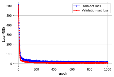
6. Visualize the result

loss = history.history['mean_squared_error']
val_loss = history.history['val_mean_squared_error']

x_len = np.arange(len(loss))

plt.plot(x_len, loss, marker='.', c='blue', label="Train-set loss.")
plt.plot(x_len, val_loss, marker='.', c='red', label="Validation-set loss.")

plt.legend(loc='upper right')
plt.grid()
plt.xlabel('epoch')
plt.ylabel('Loss(MSE)')
plt.show()

 

loss = history.history['mean_squared_error']
val_loss = history.history['val_mean_squared_error']

x_len = np.arange(len(loss))

# epoch 200 ~ epoch 1000
plt.plot(x_len[200:], loss[200:], marker='.', c='blue', label="Train-set loss.")
plt.plot(x_len[200:], val_loss[200:], marker='.', c='red', label="Validation-set loss.")

plt.legend(loc='upper right')
plt.grid()
plt.xlabel('epoch')
plt.ylabel('Loss(MSE)')
plt.show()

 

---

* Predict test data / new data

# predict test data
model.predict(test_data)

# predict new data
sample_data = np.array([[0.02731, 0.0, 7.07, 0.0, 0.469, 6.421, 78.9, 4.9671, 2.0, 242.0, 17.8, 396.90, 9.14]])
sample_data = sc.transform(sample_data) # "transform" the sample data with fitted scaler (no "fit", just "transform")
model.predict(sample_data)